A < B  processA takes input from fileB
A > B  processA wirte on fileB
A >> B processA appends to fileB
A | B  output of A is input to B
A << B take input from following lines(B represents text)
Tips:'|' is similar to Perl in which represents a pipe
UNIF2用法介绍
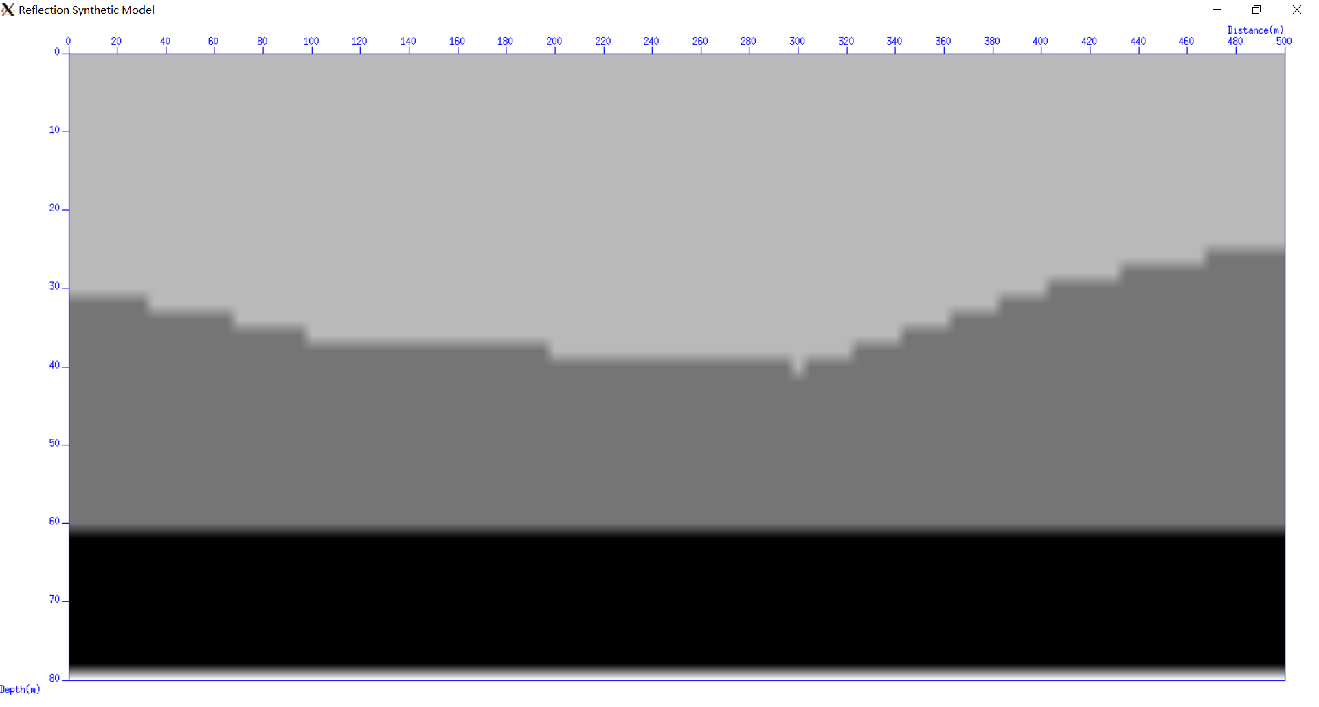
UNIF2 - generate a 2-D UNIFormly sampled velocity profile from a layered model. In each layer, velocity is a linear function of position.
格式
unif2 < infile > outfile [parameters]
必要参数: none
可选参数: ninf=5 分界面数量 nx=100 x轴采样个数 (2nd dimension) nz=100 z轴采样个数 (1st dimension) dx=10 x sampling interval dz=10 z sampling interval
npmax=201 maximum number of points on interfaces
fx=0.0 first x sample fz=0.0 first z sample
x0=0.0,0.0,…, distance x at which v00 is specified z0=0.0,0.0,…, depth z at which v00 is specified v00=1500,2000,2500…, velocity at each x0,z0 (m/sec)
dvdx=0.0,0.0,…, derivative of velocity with distance x (dv/dx) dvdz=0.0,0.0,…, derivative of velocity with depth z (dv/dz)
method=linear for linear interpolation of interface =mono for monotonic cubic interpolation of interface =akima for Akima’s cubic interpolation of interface =spline for cubic spline interpolation of interface
tfile= =testfilename if set, a sample input dataset is output to “testfilename”.
Required Parameters:
n1                      number of samples in 1st (fast) dimension

Optional Parameters:
d1=1.0          sampling interval in 1st dimension
f1=0.0          first sample in 1st dimension
n2=all          number of samples in 2nd (slow) dimension
d2=1.0          sampling interval in 2nd dimension
f2=0.0          first sample in 2nd dimension
mpicks=/dev/tty         file to save mouse picks in
perc=100.0              percentile used to determine clip
clip=(perc percentile) clip used to determine bclip and wclip
bperc=perc              percentile for determining black clip value
wperc=100.0-perc        percentile for determining white clip value
bclip=clip              data values outside of [bclip,wclip] are clipped
wclip=-clip             data values outside of [bclip,wclip] are clipped
balance=0               bclip & wclip individually
                        =1 set them to the same abs value
                          if specified via perc (avoids colorbar skew)
cmap=hsv\'n\' or rgb\'m\'      \'n\' is a number from 0 to 13
                               \'m\' is a number from 0 to 11
                               cmap=rgb0 is equal to cmap=gray
                               cmap=hsv1 is equal to cmap=hue
                               (compatibility to older versions)
legend=0               =1 display the color scale
units=         unit label for legend
legendfont=times_roman10    font name for title
verbose=1              =1 for info printed on stderr (0 for no info)
xbox=50                x in pixels of upper left corner of window
ybox=50                y in pixels of upper left corner of window
wbox=550               width in pixels of window
hbox=700               height in pixels of window
lwidth=16              colorscale (legend) width in pixels
lheight=hbox/3 colorscale (legend) height in pixels
lx=3                   colorscale (legend) x-position in pixels
ly=(hbox-lheight)/3   colorscale (legend) y-position in pixels
x1beg=x1min            value at which axis 1 begins
x1end=x1max            value at which axis 1 ends
d1num=0.0              numbered tic interval on axis 1 (0.0 for automatic)
f1num=x1min            first numbered tic on axis 1 (used if d1num not 0.0)
n1tic=1                number of tics per numbered tic on axis 1
grid1=none             grid lines on axis 1 - none, dot, dash, or solid
label1=                label on axis 1
x2beg=x2min            value at which axis 2 begins
x2end=x2max            value at which axis 2 ends
d2num=0.0              numbered tic interval on axis 2 (0.0 for automatic)
f2num=x2min            first numbered tic on axis 2 (used if d2num not 0.0)
n2tic=1                number of tics per numbered tic on axis 2
grid2=none             grid lines on axis 2 - none, dot, dash, or solid
label2=                label on axis 2
labelfont=Erg14        font name for axes labels
title=         title of plot
titlefont=Rom22        font name for title
windowtitle=ximage     title on window
labelcolor=blue        color for axes labels
titlecolor=red color for title
gridcolor=blue color for grid lines
style=seismic          normal (axis 1 horizontal, axis 2 vertical) or
                       seismic (axis 1 vertical, axis 2 horizontal)
blank=0                This indicates what portion of the lower range
                       to blank out (make the background color).  The
                       value should range from 0 to 1.
plotfile=plotfile.ps  filename for interactive ploting (P)
curve=curve1,curve2,...  file(s) containing points to draw curve(s)
npair=n1,n2,n2,...            number(s) of pairs in each file
curvecolor=color1,color2,...  color(s) for curve(s)
blockinterp=0       whether to use block interpolation (0=no, 1=yes)
Comments